Continuous Values Into Discrete Intervals Python
Binning Data with Pandas qcut and cut
              
            
Introduction
When dealing with continuous numeric data, it is often helpful to bin the data into multiple buckets for further analysis. There are several different terms for binning including bucketing, discrete binning, discretization or quantization. Pandas supports these approaches using the                                  cut                and                                  qcut                functions. This article will briefly describe why you may want to bin your data and how to use the pandas functions to convert continuous data to a set of discrete buckets. Like many pandas functions,                                  cut                and                                  qcut                may seem simple but there is a lot of capability packed into those functions. Even for more experience users, I think you will learn a couple of tricks that will be useful for your own analysis.
Binning
One of the most common instances of binning is done behind the scenes for you when creating a histogram. The histogram below of customer sales data, shows how a continuous set of sales numbers can be divided into discrete bins (for example: $60,000 - $70,000) and then used to group and count account instances.
Here is the code that show how we summarize 2018 Sales information for a group of customers. This representation illustrates the number of customers that have sales within certain ranges. Sample code is included in this notebook if you would like to follow along.
                                    import                  pandas                  as                  pd                  import                  numpy                  as                  np                  import                  seaborn                  as                  sns                  sns                  .                  set_style                  (                  'whitegrid'                  )                  raw_df                  =                  pd                  .                  read_excel                  (                  '2018_Sales_Total.xlsx'                  )                  df                  =                  raw_df                  .                  groupby                  ([                  'account number'                  ,                  'name'                  ])[                  'ext price'                  ]                  .                  sum                  ()                  .                  reset_index                  ()                  df                  [                  'ext price'                  ]                  .                  plot                  (                  kind                  =                  'hist'                  )                                              
              
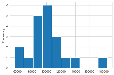
There are many other scenarios where you may want to define your own bins. In the example above, there are 8 bins with data. What if we wanted to divide our customers into 3, 4 or 5 groupings? That's where pandas                                  qcut                and                                  cut                come into play. These functions sound similar and perform similar binning functions but have differences that might be confusing to new users. They also have several options that can make them very useful for day to day analysis. The rest of the article will show what their differences are and how to use them.
qcut
The pandas documentation describes                                  qcut                as a "Quantile-based discretization function." This basically means that                                  qcut                tries to divide up the underlying data into equal sized bins. The function defines the bins using percentiles based on the distribution of the data, not the actual numeric edges of the bins.
If you have used the pandas                                  describe                function, you have already seen an example of the underlying concepts represented by                                  qcut                :
                                    df                  [                  'ext price'                  ]                  .                  describe                  ()                                                                  count                  20.000000                  mean                  101711.287500                  std                  27037.449673                  min                  55733.050000                  25                  %                  89137.707500                  50                  %                  100271.535000                  75                  %                  110132.552500                  max                  184793.700000                  Name                  :                  ext                  price                  ,                  dtype                  :                  float64                              Keep in mind the values for the 25%, 50% and 75% percentiles as we look at using                                  qcut                directly.
The simplest use of                                  qcut                is to define the number of quantiles and let pandas figure out how to divide up the data. In the example below, we tell pandas to create 4 equal sized groupings of the data.
                                    pd                  .                  qcut                  (                  df                  [                  'ext price'                  ],                  q                  =                  4                  )                                                                  0                  (                  55733.049000000006                  ,                  89137.708                  ]                  1                  (                  89137.708                  ,                  100271.535                  ]                  2                  (                  55733.049000000006                  ,                  89137.708                  ]                  ....                  17                  (                  110132.552                  ,                  184793.7                  ]                  18                  (                  100271.535                  ,                  110132.552                  ]                  19                  (                  100271.535                  ,                  110132.552                  ]                  Name                  :                  ext                  price                  ,                  dtype                  :                  category                  Categories                  (                  4                  ,                  interval                  [                  float64                  ]):                  [(                  55733.049000000006                  ,                  89137.708                  ]                  <                  (                  89137.708                  ,                  100271.535                  ]                  <                  (                  100271.535                  ,                  110132.552                  ]                  <                  (                  110132.552                  ,                  184793.7                  ]]                              The result is a categorical series representing the sales bins. Because we asked for quantiles with                                  q=4                the bins match the percentiles from the                                  describe                function.
A common use case is to store the bin results back in the original dataframe for future analysis. For this example, we will create 4 bins (aka quartiles) and 10 bins (aka deciles) and store the results back in the original dataframe:
                                    df                  [                  'quantile_ex_1'                  ]                  =                  pd                  .                  qcut                  (                  df                  [                  'ext price'                  ],                  q                  =                  4                  )                  df                  [                  'quantile_ex_2'                  ]                  =                  pd                  .                  qcut                  (                  df                  [                  'ext price'                  ],                  q                  =                  10                  ,                  precision                  =                  0                  )                  df                  .                  head                  ()                              | account number | name | ext price | quantile_ex_1 | quantile_ex_2 | |
|---|---|---|---|---|---|
| 0 | 141962 | Herman LLC | 63626.03 | (55733.049000000006, 89137.708] | (55732.0, 76471.0] | 
| 1 | 146832 | Kiehn-Spinka | 99608.77 | (89137.708, 100271.535] | (95908.0, 100272.0] | 
| 2 | 163416 | Purdy-Kunde | 77898.21 | (55733.049000000006, 89137.708] | (76471.0, 87168.0] | 
| 3 | 218895 | Kulas Inc | 137351.96 | (110132.552, 184793.7] | (124778.0, 184794.0] | 
| 4 | 239344 | Stokes LLC | 91535.92 | (89137.708, 100271.535] | (90686.0, 95908.0] | 
You can see how the bins are very different between                                  quantile_ex_1                and                                  quantile_ex_2                . I also introduced the use of                                  precision                to define how many decimal points to use for calculating the bin precision.
The other interesting view is to see how the values are distributed across the bins using                                  value_counts                :
                                    df                  [                  'quantile_ex_1'                  ]                  .                  value_counts                  ()                                                                  (                  110132.552                  ,                  184793.7                  ]                  5                  (                  100271.535                  ,                  110132.552                  ]                  5                  (                  89137.708                  ,                  100271.535                  ]                  5                  (                  55733.049000000006                  ,                  89137.708                  ]                  5                  Name                  :                  quantile_ex_1                  ,                  dtype                  :                  int64                              Now, for the second column:
                                    df                  [                  'quantile_ex_2'                  ]                  .                  value_counts                  ()                                                                  (                  124778.0                  ,                  184794.0                  ]                  2                  (                  112290.0                  ,                  124778.0                  ]                  2                  (                  105938.0                  ,                  112290.0                  ]                  2                  (                  103606.0                  ,                  105938.0                  ]                  2                  (                  100272.0                  ,                  103606.0                  ]                  2                  (                  95908.0                  ,                  100272.0                  ]                  2                  (                  90686.0                  ,                  95908.0                  ]                  2                  (                  87168.0                  ,                  90686.0                  ]                  2                  (                  76471.0                  ,                  87168.0                  ]                  2                  (                  55732.0                  ,                  76471.0                  ]                  2                  Name                  :                  quantile_ex_2                  ,                  dtype                  :                  int64                              This illustrates a key concept. In each case, there are an equal number of observations in each bin. Pandas does the math behind the scenes to figure out how wide to make each bin. For instance, in                                  quantile_ex_1                the range of the first bin is 74,661.15 while the second bin is only 9,861.02 (110132 - 100271).
One of the challenges with this approach is that the bin labels are not very easy to explain to an end user. For instance, if we wanted to divide our customers into 5 groups (aka quintiles) like an airline frequent flier approach, we can explicitly label the bins to make them easier to interpret.
                                    bin_labels_5                  =                  [                  'Bronze'                  ,                  'Silver'                  ,                  'Gold'                  ,                  'Platinum'                  ,                  'Diamond'                  ]                  df                  [                  'quantile_ex_3'                  ]                  =                  pd                  .                  qcut                  (                  df                  [                  'ext price'                  ],                  q                  =                  [                  0                  ,                  .                  2                  ,                  .                  4                  ,                  .                  6                  ,                  .                  8                  ,                  1                  ],                  labels                  =                  bin_labels_5                  )                  df                  .                  head                  ()                              | account number | name | ext price | quantile_ex_1 | quantile_ex_2 | quantile_ex_3 | |
|---|---|---|---|---|---|---|
| 0 | 141962 | Herman LLC | 63626.03 | (55733.049000000006, 89137.708] | (55732.0, 76471.0] | Bronze | 
| 1 | 146832 | Kiehn-Spinka | 99608.77 | (89137.708, 100271.535] | (95908.0, 100272.0] | Gold | 
| 2 | 163416 | Purdy-Kunde | 77898.21 | (55733.049000000006, 89137.708] | (76471.0, 87168.0] | Bronze | 
| 3 | 218895 | Kulas Inc | 137351.96 | (110132.552, 184793.7] | (124778.0, 184794.0] | Diamond | 
| 4 | 239344 | Stokes LLC | 91535.92 | (89137.708, 100271.535] | (90686.0, 95908.0] | Silver | 
In the example above, I did somethings a little differently. First, I explicitly defined the range of quantiles to use:                                  q=[0, .2, .4, .6, .8, 1]                . I also defined the labels                                  labels=bin_labels_5                to use when representing the bins.
Let's check the distribution:
                                    df                  [                  'quantile_ex_3'                  ]                  .                  value_counts                  ()                                                                  Diamond                  4                  Platinum                  4                  Gold                  4                  Silver                  4                  Bronze                  4                  Name                  :                  quantile_ex_3                  ,                  dtype                  :                  int64                              As expected, we now have an equal distribution of customers across the 5 bins and the results are displayed in an easy to understand manner.
One important item to keep in mind when using                                  qcut                is that the quantiles must all be less than 1. Here are some examples of distributions. In most cases it's simpler to just define                                  q                as an integer:
- terciles:                  
q=[0, 1/3, 2/3, 1]orq=3 - quintiles:                  
q=[0, .2, .4, .6, .8, 1]orq=5 - sextiles:                  
q=[0, 1/6, 1/3, .5, 2/3, 5/6, 1]orq=6 
One question you might have is, how do I know what ranges are used to identify the different bins? You can use                                  retbins=True                to return the bin labels. Here's a handy snippet of code to build a quick reference table:
                                    results                  ,                  bin_edges                  =                  pd                  .                  qcut                  (                  df                  [                  'ext price'                  ],                  q                  =                  [                  0                  ,                  .                  2                  ,                  .                  4                  ,                  .                  6                  ,                  .                  8                  ,                  1                  ],                  labels                  =                  bin_labels_5                  ,                  retbins                  =                  True                  )                  results_table                  =                  pd                  .                  DataFrame                  (                  zip                  (                  bin_edges                  ,                  bin_labels_5                  ),                  columns                  =                  [                  'Threshold'                  ,                  'Tier'                  ])                              | Threshold | Tier | |
|---|---|---|
| 0 | 55733.050 | Bronze | 
| 1 | 87167.958 | Silver | 
| 2 | 95908.156 | Gold | 
| 3 | 103606.970 | Platinum | 
| 4 | 112290.054 | Diamond | 
Here is another trick that I learned while doing this article. If you try                                  df.describe                on categorical values, you get different summary results:
                                    df                  .                  describe                  (                  include                  =                  'category'                  )                              | quantile_ex_1 | quantile_ex_2 | quantile_ex_3 | |
|---|---|---|---|
| count | 20 | 20 | 20 | 
| unique | 4 | 10 | 5 | 
| top | (110132.552, 184793.7] | (124778.0, 184794.0] | Diamond | 
| freq | 5 | 2 | 4 | 
I think this is useful and also a good summary of how                                  qcut                works.
While we are discussing                                  describe                we can using the                                  percentiles                argument to define our percentiles using the same format we used for                                  qcut                :
                                    df                  .                  describe                  (                  percentiles                  =                  [                  0                  ,                  1                  /                  3                  ,                  2                  /                  3                  ,                  1                  ])                              | account number | ext price | |
|---|---|---|
| count | 20.000000 | 20.000000 | 
| mean | 476998.750000 | 101711.287500 | 
| std | 231499.208970 | 27037.449673 | 
| min | 141962.000000 | 55733.050000 | 
| 0% | 141962.000000 | 55733.050000 | 
| 33.3% | 332759.333333 | 91241.493333 | 
| 50% | 476006.500000 | 100271.535000 | 
| 66.7% | 662511.000000 | 104178.580000 | 
| 100% | 786968.000000 | 184793.700000 | 
| max | 786968.000000 | 184793.700000 | 
There is one minor note about this functionality. Passing 0 or 1, just means that the 0% will be the same as the min and 100% will be same as the max. I also learned that the 50th percentile will always be included, regardless of the values passed.
Before we move on to describing                                  cut                , there is one more potential way that we can label our bins. Instead of the bin ranges or custom labels, we can return integers by passing                                  labels=False              
                                    df                  [                  'quantile_ex_4'                  ]                  =                  pd                  .                  qcut                  (                  df                  [                  'ext price'                  ],                  q                  =                  [                  0                  ,                  .                  2                  ,                  .                  4                  ,                  .                  6                  ,                  .                  8                  ,                  1                  ],                  labels                  =                  False                  ,                  precision                  =                  0                  )                  df                  .                  head                  ()                              | account number | name | ext price | quantile_ex_1 | quantile_ex_2 | quantile_ex_3 | quantile_ex_4 | |
|---|---|---|---|---|---|---|---|
| 0 | 141962 | Herman LLC | 63626.03 | (55733.049000000006, 89137.708] | (55732.0, 76471.0] | Bronze | 0 | 
| 1 | 146832 | Kiehn-Spinka | 99608.77 | (89137.708, 100271.535] | (95908.0, 100272.0] | Gold | 2 | 
| 2 | 163416 | Purdy-Kunde | 77898.21 | (55733.049000000006, 89137.708] | (76471.0, 87168.0] | Bronze | 0 | 
| 3 | 218895 | Kulas Inc | 137351.96 | (110132.552, 184793.7] | (124778.0, 184794.0] | Diamond | 4 | 
| 4 | 239344 | Stokes LLC | 91535.92 | (89137.708, 100271.535] | (90686.0, 95908.0] | Silver | 1 | 
Personally, I think using                                  bin_labels                is the most useful scenario but there could be cases where the integer response might be helpful so I wanted to explicitly point it out.
cut
Now that we have discussed how to use                                  qcut                , we can show how                                  cut                is different. Many of the concepts we discussed above apply but there are a couple of differences with the usage of                                  cut                .
The major distinction is that                                  qcut                will calculate the size of each bin in order to make sure the distribution of data in the bins is equal. In other words, all bins will have (roughly) the same number of observations but the bin range will vary.
On the other hand,                                  cut                is used to specifically define the bin edges. There is no guarantee about the distribution of items in each bin. In fact, you can define bins in such a way that no items are included in a bin or nearly all items are in a single bin.
In real world examples, bins may be defined by business rules. For a frequent flier program, 25,000 miles is the silver level and that does not vary based on year to year variation of the data. If we want to define the bin edges (25,000 - 50,000, etc) we would use                                  cut                . We can also use                                  cut                to define bins that are of constant size and let pandas figure out how to define those bin edges.
Some examples should make this distinction clear.
For the sake of simplicity, I am removing the previous columns to keep the examples short:
                                    df                  =                  df                  .                  drop                  (                  columns                  =                  [                  'quantile_ex_1'                  ,                  'quantile_ex_2'                  ,                  'quantile_ex_3'                  ,                  'quantile_ex_4'                  ])                              For the first example, we can cut the data into 4 equal bin sizes. Pandas will perform the math behind the scenes to determine how to divide the data set into these 4 groups:
                                    pd                  .                  cut                  (                  df                  [                  'ext price'                  ],                  bins                  =                  4                  )                                                                  0                  (                  55603.989                  ,                  87998.212                  ]                  1                  (                  87998.212                  ,                  120263.375                  ]                  2                  (                  55603.989                  ,                  87998.212                  ]                  3                  (                  120263.375                  ,                  152528.538                  ]                  4                  (                  87998.212                  ,                  120263.375                  ]                  ....                  14                  (                  87998.212                  ,                  120263.375                  ]                  15                  (                  120263.375                  ,                  152528.538                  ]                  16                  (                  87998.212                  ,                  120263.375                  ]                  17                  (                  87998.212                  ,                  120263.375                  ]                  18                  (                  87998.212                  ,                  120263.375                  ]                  19                  (                  87998.212                  ,                  120263.375                  ]                  Name                  :                  ext                  price                  ,                  dtype                  :                  category                  Categories                  (                  4                  ,                  interval                  [                  float64                  ]):                  [(                  55603.989                  ,                  87998.212                  ]                  <                  (                  87998.212                  ,                  120263.375                  ]                  <                  (                  120263.375                  ,                  152528.538                  ]                  <                  (                  152528.538                  ,                  184793.7                  ]]                              Let's look at the distribution:
                                    pd                  .                  cut                  (                  df                  [                  'ext price'                  ],                  bins                  =                  4                  )                  .                  value_counts                  ()                                                                  (                  87998.212                  ,                  120263.375                  ]                  12                  (                  55603.989                  ,                  87998.212                  ]                  5                  (                  120263.375                  ,                  152528.538                  ]                  2                  (                  152528.538                  ,                  184793.7                  ]                  1                  Name                  :                  ext                  price                  ,                  dtype                  :                  int64                              The first thing you'll notice is that the bin ranges are all about 32,265 but that the distribution of bin elements is not equal. The bins have a distribution of 12, 5, 2 and 1 item(s) in each bin. In a nutshell, that is the essential difference between                                  cut                and                                  qcut                .
Info
                  If you want equal distribution of the items in your bins, use                                      qcut                  . If you want to define your own numeric bin ranges, then use                                      cut                  .
Before going any further, I wanted to give a quick refresher on interval notation. In the examples above, there have been liberal use of ()'s and []'s to denote how the bin edges are defined. For those of you (like me) that might need a refresher on interval notation, I found this simple site very easy to understand.
To bring this home to our example, here is a diagram based off the example above:
                
              
When using cut, you may be defining the exact edges of your bins so it is important to understand if the edges include the values or not. Depending on the data set and specific use case, this may or may not be a big issue. It can certainly be a subtle issue you do need to consider.
To bring it into perspective, when you present the results of your analysis to others, you will need to be clear whether an account with 70,000 in sales is a silver or gold customer.
Here is an example where we want to specifically define the boundaries of our 4 bins by defining the                                  bins                parameter.
                                    cut_labels_4                  =                  [                  'silver'                  ,                  'gold'                  ,                  'platinum'                  ,                  'diamond'                  ]                  cut_bins                  =                  [                  0                  ,                  70000                  ,                  100000                  ,                  130000                  ,                  200000                  ]                  df                  [                  'cut_ex1'                  ]                  =                  pd                  .                  cut                  (                  df                  [                  'ext price'                  ],                  bins                  =                  cut_bins                  ,                  labels                  =                  cut_labels_4                  )                              | account number | name | ext price | cut_ex1 | |
|---|---|---|---|---|
| 0 | 141962 | Herman LLC | 63626.03 | silver | 
| 1 | 146832 | Kiehn-Spinka | 99608.77 | gold | 
| 2 | 163416 | Purdy-Kunde | 77898.21 | gold | 
| 3 | 218895 | Kulas Inc | 137351.96 | diamond | 
| 4 | 239344 | Stokes LLC | 91535.92 | gold | 
One of the challenges with defining the bin ranges with cut is that it can be cumbersome to create the list of all the bin ranges. There are a couple of shortcuts we can use to compactly create the ranges we need.
First, we can use                                  numpy.linspace                to create an equally spaced range:
                                    pd                  .                  cut                  (                  df                  [                  'ext price'                  ],                  bins                  =                  np                  .                  linspace                  (                  0                  ,                  200000                  ,                  9                  ))                                                                  0                  (                  50000.0                  ,                  75000.0                  ]                  1                  (                  75000.0                  ,                  100000.0                  ]                  2                  (                  75000.0                  ,                  100000.0                  ]                  ....                  18                  (                  100000.0                  ,                  125000.0                  ]                  19                  (                  100000.0                  ,                  125000.0                  ]                  Name                  :                  ext                  price                  ,                  dtype                  :                  category                  Categories                  (                  8                  ,                  interval                  [                  float64                  ]):                  [(                  0.0                  ,                  25000.0                  ]                  <                  (                  25000.0                  ,                  50000.0                  ]                  <                  (                  50000.0                  ,                  75000.0                  ]                  <                  (                  75000.0                  ,                  100000.0                  ]                  <                  (                  100000.0                  ,                  125000.0                  ]                  <                  (                  125000.0                  ,                  150000.0                  ]                  <                  (                  150000.0                  ,                  175000.0                  ]                  <                  (                  175000.0                  ,                  200000.0                  ]]                              Numpy's linspace is a simple function that provides an array of evenly spaced numbers over a user defined range. In this example, we want 9 evenly spaced cut points between 0 and 200,000. Astute readers may notice that we have 9 numbers but only 8 categories. If you map out the actual categories, it should make sense why we ended up with 8 categories between 0 and 200,000. In all instances, there is one less category than the number of cut points.
The other option is to use                                  numpy.arange                which offers similar functionality. I found this article a helpful guide in understanding both functions. I recommend trying both approaches and seeing which one works best for your needs.
There is one additional option for defining your bins and that is using pandas                                  interval_range                . I had to look at the pandas documentation to figure out this one. It is a bit esoteric but I think it is good to include it.
The                                  interval_range                offers a lot of flexibility. For instance, it can be used on date ranges as well numerical values. Here is a numeric example:
                                    pd                  .                  interval_range                  (                  start                  =                  0                  ,                  freq                  =                  10000                  ,                  end                  =                  200000                  ,                  closed                  =                  'left'                  )                                                                  IntervalIndex                  ([[                  0                  ,                  10000                  ),                  [                  10000                  ,                  20000                  ),                  [                  20000                  ,                  30000                  ),                  [                  30000                  ,                  40000                  ),                  [                  40000                  ,                  50000                  )                  ...                  [                  150000                  ,                  160000                  ),                  [                  160000                  ,                  170000                  ),                  [                  170000                  ,                  180000                  ),                  [                  180000                  ,                  190000                  ),                  [                  190000                  ,                  200000                  )],                  closed                  =                  'left'                  ,                  dtype                  =                  'interval[int64]'                  )                              There is a downside to using                                  interval_range                . You can not define custom labels.
                                    interval_range                  =                  pd                  .                  interval_range                  (                  start                  =                  0                  ,                  freq                  =                  10000                  ,                  end                  =                  200000                  )                  df                  [                  'cut_ex2'                  ]                  =                  pd                  .                  cut                  (                  df                  [                  'ext price'                  ],                  bins                  =                  interval_range                  ,                  labels                  =                  [                  1                  ,                  2                  ,                  3                  ])                  df                  .                  head                  ()                              | account number | name | ext price | cut_ex1 | cut_ex2 | |
|---|---|---|---|---|---|
| 0 | 141962 | Herman LLC | 63626.03 | gold | (60000, 70000] | 
| 1 | 146832 | Kiehn-Spinka | 99608.77 | silver | (90000, 100000] | 
| 2 | 163416 | Purdy-Kunde | 77898.21 | silver | (70000, 80000] | 
| 3 | 218895 | Kulas Inc | 137351.96 | diamond | (130000, 140000] | 
| 4 | 239344 | Stokes LLC | 91535.92 | silver | (90000, 100000] | 
As shown above, the                                  labels                parameter is ignored when using the                                  interval_range                .
In my experience, I use a custom list of bin ranges or                                  linspace                if I have a large number of bins.
One of the differences between                                  cut                and                                  qcut                is that you can also use the                                  include_lowest                paramete to define whether or not the first bin should include all of the lowest values. Finally, passing                                  right=False                will alter the bins to exclude the right most item. Because                                  cut                allows much more specificity of the bins, these parameters can be useful to make sure the intervals are defined in the manner you expect.
The rest of the                                  cut                functionality is similar to                                  qcut                . We can return the bins using                                  retbins=True                or adjust the precision using the                                  precision                argument.
One final trick I want to cover is that                                  value_counts                includes a shortcut for binning and counting the data. It is somewhat analogous to the way                                  describe                can be a shortcut for                                  qcut                .
If we want to bin a value into 4 bins and count the number of occurences:
                                    df                  [                  'ext price'                  ]                  .                  value_counts                  (                  bins                  =                  4                  ,                  sort                  =                  False                  )                                                                  (                  55603.988000000005                  ,                  87998.212                  ]                  5                  (                  87998.212                  ,                  120263.375                  ]                  12                  (                  120263.375                  ,                  152528.538                  ]                  2                  (                  152528.538                  ,                  184793.7                  ]                  1                  Name                  :                  ext                  price                  ,                  dtype                  :                  int64                              By defeault                                  value_counts                will sort with the highest value first. By passing                                  sort=False                the bins will be sorted by numeric order which can be a helpful view.
Summary
The concept of breaking continuous values into discrete bins is relatively straightforward to understand and is a useful concept in real world analysis. Fortunately, pandas provides the                                  cut                and                                  qcut                functions to make this as simple or complex as you need it to be. I hope this article proves useful in understanding these pandas functions. Please feel free to comment below if you have any questions.
Updates
- 29-October-2019: Modified to include                  
value_countsshortcut for binning and counting the data. - 17-December-2019: Published article on natural breaks which leverages these concepts and provides another useful method for binning numbers.
 
credits
Photo by Radek Grzybowski on Unsplash
Source: https://pbpython.com/pandas-qcut-cut.html
0 Response to "Continuous Values Into Discrete Intervals Python"
Post a Comment